Riemannian distance for SPD circulant matrices
Or slicing cones
I was working on some homework for a course on Geometric Deep Learning. The context was differential geometry, more specifically the manifold of Symmetric Positive Definite (SPD) matrices. The exercise had us thinking about a notion of distance for this manifold. It also was presenting it as an example of the algebraic concept of a convex cone. I was left wondering: where do circulant matrices live in all of this?
SPD matrices
If you end up on this page, I take it for granted you know what a symmetric matrix is. As for the Positive Definite part, the way I think about them is like a “stretching” operator: feed it any vector, and this thing will:
- rotate it to “align it” to an orthogonal basis;
- stretch/scale every component by a strictly positive number;
- undo the rotation you did at the beginning. Importantly, an positive definite matrix has strictly positive determinant.
More info is on Wikipedia, of course.
You may find SPD matrices in the following contexts:
- as covariance matrices (if it is a sample covariance, you may need “enough” samples, so that it is not rank deficient);
- as metric tensors, once you specify some coordinate system;
- as Gram matrices, in the context of kernel methods;
- and, I assume, many more.
The manifold of SPD matrices
Imagine an \(n\times n\) matrix \(\mathcal{M}\) that is symmetric and positive definite. Due to its symmetry, you only actually need to specify \(n(n+1)/2\) elements to characterize the matrix. You can then think of this matrix as a point in the space \(\mathbb{R}^{n(n+1)/2}\). The set of all such points that correspond to a symmetric positive definite matrix forms a manifold. It is possible to endow this manifold with a metric, that is, a way to “measure distance” between two of its points, thus creating a Riemannian manifold. We call this manifold \(\mathcal{S}_{++}^n\).
A careful discussion of Riemannian manifolds is a bit outside of my capabilities, but resources are plentiful if you crave some big boy maths.
It is instructive and amusing to check what this manifold may look like in practice. Choose \(n=2\), so that matrices (which are symmetric!) are of the type
\[\mathcal{M} = \begin{pmatrix} x & z \\ z & y \end{pmatrix}.\]Additionally, we need to satisfy the requirements
\[\det \mathcal{M} = xy - z^2 >0, \quad x>0, \quad y>0.\]These are needed for the positive-definiteness requirement. The matrix \(\mathcal{M}\) above can be represented as the point \((x, y, z)\in \mathbb{R}^3\). We can think of the manifold as the following subset of \(\mathbb{R}^3\):
\[\mathcal{S}_{++}^2 = \{(x, y, z) \in \mathbb{R}^3 | xy-z^2>0, x>0, y>0\}.\]Feed this to matplotlib, and you get this:

This really looks like a geometric cone, and it also happens to be an algebraic cone.
Distance between SPD matrices
One can define a notion of distance between two SPD matrices \(P, Q \in \mathcal{S}_{++}^n\), as done in this paper: The formula looks like this:
\[d(P, Q) = \sqrt{\sum_{i=1}^n \ln^2 \lambda_i(P, Q)},\]where \(\lambda_i(P, Q)\) denotes the \(i\)-th eigenvalue that can be obtained by solving the equation
\[\det(\lambda P - Q) = 0.\]Geodesics
Similarly, we can define a geodesic between two SPD matrices, \(P, Q \in \mathcal{S}_{++}^n\), with the following formula:
\[\gamma(t) = P^{1/2}(P^{-1/2}QP^{-1/2})^tP^{1/2}, \quad t\in[0,1].\]For any \(t\in[0, 1]\), \(\gamma(t)\) is an SPD matrix. Here is some JAX code to get this geodesic:
import jax
from jax import numpy as jnp
from typing import Callable
def get_geodesic(P: jax.Array, Q: jax.Array) -> Callable:
Op, Sp, OpT = jnp.linalg.svd(P, hermitian=True)
Phalf = (Op * jnp.sqrt(Sp)) @ OpT
Pmhalf = (Op * (1/jnp.sqrt(Sp))) @ OpT
pow = Pmhalf @ Q @ Pmhalf
Opow, Spow, OpowT = jnp.linalg.svd(pow, hermitian=True)
def gamma(t: float) -> jax.Array:
return Phalf @ ((Opow * (Spow**t)) @ OpowT) @ Phalf
return gamma
# example usage
P1 = jnp.array([ [3, 1], [1, 4]] )
Q1 = jnp.array([ [1, 0], [0, 1]] )
gamma = get_geodesic(P1, Q1)
times = jnp.linspace(0, 1, 100)
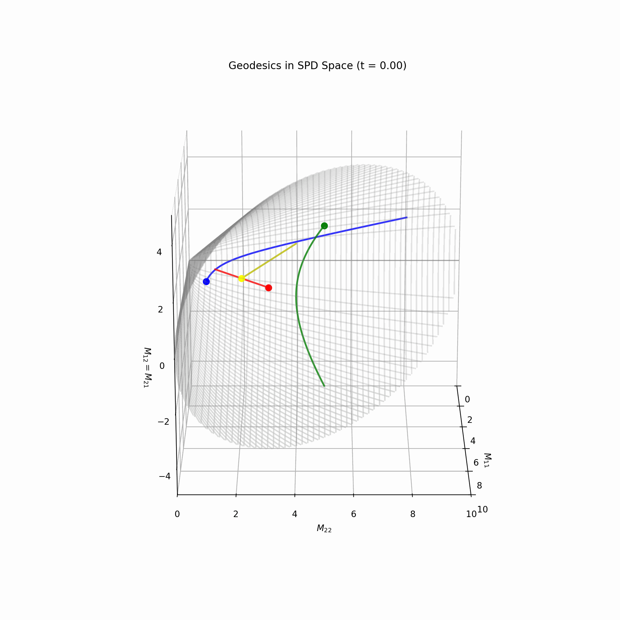
path = vmap(gamma)(times)Using this code and a bit of 3D plotting, we get this gif, showing a few geodesics in the \(\mathcal{S}_{++}^2\) manifold.
Circulant matrices
Now, let’s move to circulant matrices that also happen to be SPD.
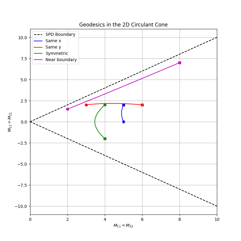
Let us start from the case \(n=2\). A 2 by 2, positive definite circulant matrix can be written as
\[\mathcal{M} = \begin{pmatrix} x & z \\ z & x \end{pmatrix},\]with \(x>0\) and \(|z| < x\). This is a manifold, too! I will call it \(\mathcal{C}_{++}^2\); this is a 2D manifold (one fewer dimension than \(\mathcal{S}_{++}^2\)). Specifically, it can be visualized as a slice of the cone above, obtained by intersecting it with the plane \(x=y\). This is, again, a cone (at least algebraically speaking; I guess it is also geometrically a 2D cone). We can now visualize the geodesics between circulant matrices on a 2D plane.
Geodesic formula for \(\mathcal{C}_{++}^n\)
We can just reuse the geodesic formula for \(\mathcal{S}_{++}^n\) and specialize it to the submanifold of circulant matrices. Consider \(P, Q \in \mathcal{C}_{++}^n\); these are diagonalized by the DFT matrix, \(\mathcal{F}\):
\[P = \mathcal{F} \Lambda_P \mathcal{F}^{-1}, \quad Q = \mathcal{F} \Lambda_Q \mathcal{F}^{-1}.\]Then, we get an easier expression for \(\gamma: [0, 1] \to \mathcal{C}_{++}^n\):
\[\gamma(t) = \mathcal{F} \frac{\Lambda_Q^t}{\Lambda_P^{t-1}} \mathcal{F}^{-1},\]where the ratio and the power operation are understood to happen elementwise. As a sanity check, we see that \(\gamma(0) = P\) and \(\gamma(1) = Q\), as expected. The code for this geodesic is a tiny bit cleaner, as well:
import jax
from jax import numpy as jnp, vmap
from typing import Callable


def get_circ_geodesic(P: jax.Array, Q: jax.Array) -> Callable:
    lp = jnp.fft.rfft(P)
    lq = jnp.fft.rfft(Q)
    def gamma(t: float) -> jax.Array:
        return jnp.fft.irfft(lp**t / lq**(t-1))
    return gamma


# example usage
P1 = jnp.array([ [3, 1], [1, 3]] )
Q1 = jnp.array([ [1, 0], [0, 1]] )
gamma = get_circ_geodesic(P1, Q1)
times = jnp.linspace(0, 1, 100)
path = vmap(gamma)(times)
Distances
What about the distance between two circulant matrices? Again, we can just take the definition of distance that holds for generic SPD matrices, and use the properties of circulant matrices. We get
\[d(P, Q)^2 = \sum_i \left(\ln\frac{(\Lambda_P)_i}{(\Lambda_Q)_i}\right)^2,\]where \(\Lambda_P, \Lambda_Q\) are the spectra of the matrices \(P, Q\) (in other words, their DFT). After slight manipulation, this expression looks a lot like a usual Euclidean distance:
\[d(P, Q)^2 = \sum_i \left(\ln(\Lambda_P)_i - \ln(\Lambda_Q)_i\right)^2,\]so a sum of squared log-distances between eigenvalues.
TODO: find analogies in signal processing maybe?
Open questions
I have one question left at the moment (hopefully, more will arise). The question is: take a matrix \(P \in \mathcal{S}_{++}^n\); what is the closest matrix \(Q \in \mathcal{C}_{++}^n\)? The idea has something to do with our recent paper, where we use an ex-post circularization procedure on Gram matrices. This circularization happens by simply averaging the diagonals of the Gram matrix. At first glance, it seems like there is no other way to make a matrix circulant that would make much sense. So it would be nice to see if it just so happens that this diagonal-averaged matrix is the “orthogonal projection” of an SPD matrix onto the submanifold of circulant SPD matrices. A possible plan of attack would be to minimize the length between an arbitrary SPD matrix $P$ and a target circulant SPD matrix \(Q\). I will maybe do that in the next days.
References
A list of references:
- a definition of distance between SPD matrices: http://www.ipb.uni-bonn.de/pdfs/Forstner1999Metric.pdf
- our recent paper: https://arxiv.org/abs/2412.11521
- the code for generating the plots can be found here